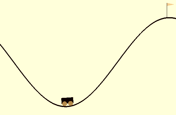
 Mountain-Car Environment Credits:OpenAI
Inverse Reinforcement Learning:
The core concept of reinforcement learning in Markov decision process revolves around the definition of reward values. The agent observes a state, proceed with an action and the environment provides the reward and the next state.

However, there are numerous cases where designing reward functions are complicated or ‘Mission Impossible’. For example, we want to train an RL agent to drive a car autonomously. The reward function can be hand-engineered, but creating such functions is often time consuming and sub-optimal. Given such reward functions, the agent may not be able to train for the given task.
In numerous scenarios like the one mentioned above, the human knows the optimal way to perform the task (Expert policy) but do not understand the underlying reward function behind the task. So, we instead think of ways to use expert human policies instead of reward functions for an agent.
The simplest of all is just copying the expert behaviour. Given expert trajectories, we design the learning process from a supervised learning perspective: Learn direct mapping from state to actions. This method is known as Behavior Cloning.
Instead of naive copying, can we recreate the reward function of the environment given expert behaviours? Yes. This approach of imitating an expert through learning the reward functions is known as Inverse Reinforcement Learning.

The first IRL algorithm (known as Linear Inverse RL) was published in a paper Algorithms for IRL (Ng & Russel 2000) in which they proposed an iterative algorithm to extract the reward function given optimal/expert behaviour policy for obtaining the goal in that particular environment. We will discuss in short what are the significant problems that Inverse RL algorithms face. But, notations first.
Notations:
- Markov decision process : $< S, А, P_{sa}, γ, R >$
- Where $S$ = finite/infinite set of states
- $A$ = action set
- $P_{sa}$ = transition probability matrix
- γ = discount factor
- R = reward function
- $π : S➝A $ is th policy function.
- $ V^{\pi}(s_t)=E[R(s_t)+R(s_{t+1})] $ Value function
- $ Q^π(s, a) = R(s) + γ * E_{s’ \sim P_{sa}}[ V^π(s’) ] $ Action value function
- $V^*(s)$ : optimal value function
- $Q^*(s, a)$ : optimal state value function
The problem is to find a reward function for an environment given optimal behavior/policy. Now, given certain basic conditions, we can easily prove the theorm mentioned below.
Theorem 1: Let $〈S, А, { Pa }, γ〉$ is known. Then, $π(s)≡a1$ is optimal if and only if for all $a∈ A-a1$ , the reward satisfies the equation $$ (P_{a1} - P_a)(I - γ P_{a1})^{-1} R ≽ 0 $$
See the problem in the above equation?
It’s the degeneracy of reward functions. Each policy has a large set of reward function for which the policy is optimal. The set even includes $R=0 ∀s∈S$. There are even more solutions other than these trivial ones. We do not want these trivial reward functions, as the agent will spend its entire lifetime iterating with 0 reward function and will not learn a thing. So how can we choose reward function from such a vast set of solutions?
Heuristics :
We use some specific heuristics.
- The natural way is to choose a reward function such that deviating from the policy on any single step must be as costly as possible. This intuition is represented in mathematical terms, as mentioned below. $$ ∑_{s∈S}( Q^π(s,a_1) - max_{a∈A-a_1}Q^π(s,a) ) $$
- If the above condition does give degenerate results, the second condition is to add a penalty coefficient, $-λ || R ||_1$ . It will make sure that the reward function remains zero in most places and non-zero at only some states with high profit.
The net reward search equation becomes: $$ Maximize ∑_i min_{π∈丌} ~ { p( V^{π*}(s’) - V^{π_i}(s’) ) } $$ $$s.t ~~ |α_i| ≤ 1, ~~~~ i =1,2,..d $$ $$ p(x)=x~when~x>0, ~else ~penalty*x $$ which can be solved with linear programming methods if reward functions are assumed to be linear.
The paper explained three possible algorithms varying only w.r.t the underlying conditions.
- Expert policy function $\pi(s)$ is known, state space $S$ is finite, and transition probabilities $P_{sa}$ are known. (Too ideal case)
- Expert policy function $\pi(s)$ is known, state space $S$ is infinite, and transition probabilities $P_{sa}$ are known. (Too ideal case)
- m expert demonstrations/ trajectories are known. Transition probabilities are not known. (The realistic case)
Algorithm flowchart:

Experiments:
I used the MountainCar-v0 environment of OpenAI gym for training and testing the algorithm.
- Expert Agent: Used Q-learning algorithm with linear approximators to train the agent for generating expert policy.(This approach is used in numerous imitation learning problems as it becomes difficult for humans to generate expert policies in simulated environments as Mountain Car.)
- Specifics: Detailed specs can be found in the slides.
Refer to the github repository for code and more details.
